Introduction
In part one of this series, we explored differences between DSE Graph 5.x and 6.0-6.7 regarding how it partitions edges and vertices in Cassandra, and what this meant in regard to how you would go about breaking apart your supernodes in order to avoid wide partitions in your DSE cluster. In this second part, we will see how it works hands-on.
As we will see, while intermediary vertices are a solution available for breaking up supernodes in 6.7, it is less than ideal in many ways. This will prepare us for our third post, about what solving the same issue looks like in DSE Graph 6.8.
Our Approach
To aid us in our experiment, we put together some quick and dirty python code and some docker-compose files for quickly spinning up DSE Graph environments and loading in mock data.
You can find the repo here: https://github.com/Anant/dse-graph-supernode-generator
In order to confirm the effectiveness of intermediary vertices, we will create a control dataset and load it into a DSE 6.7 graph. The goal here is to set a baseline for how a wide partition can be created when there are supernodes within the graph. Then after that, we will show how the same amount of edges can be connected to the supernode, but with the wide partitions broken up using intermediary vertices.
To reproduce the experiment, you can follow the instructions in the README; for this blog post, I will just give a summary along with the results.
Trial #1: Create a Control Graph, with Supernodes and Wide-partitions
Step 1: Create schema
For this experiment, we will use a simple schema, with a single vertex person and an edge likes. Our graph will be called demo_who_likes_whom. For our experiment we just care about creating a wide-partitions caused by supernodes, so we don’t need anything complicated here: a couple of properties for our person vertex (name and info) and a simple partition key (uuid) is sufficient.
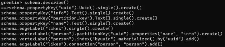
We can use CQLSH to check what’s going on inside Cassandra, thereby confirming that see that the person vertex is partitioned by the partition key we specified using the gremlin code (uuid). However, there are also some clustering columns added automatically by DSE Graph (~~property_key_id and ~~property_id).
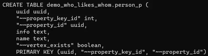
In other words, while we see some correspondence between what we do in Gremlin and what we see in the Cassandra backend, there is not a correspondence as nice and clean as what we will see in DSE 6.8.
Step 2: Send CSV data using DSE GraphLoader
When loading data into our graph, we will use DSE GraphLoader. In DSE 6.8 we can use DSE Bulk Loader instead, but this option isn’t available for DSE 6.7. DSE GraphLoader works well enough for our use case, though it is worth noting this difference as well since there are some shortcomings relative to the newer DSE Bulk Loader.
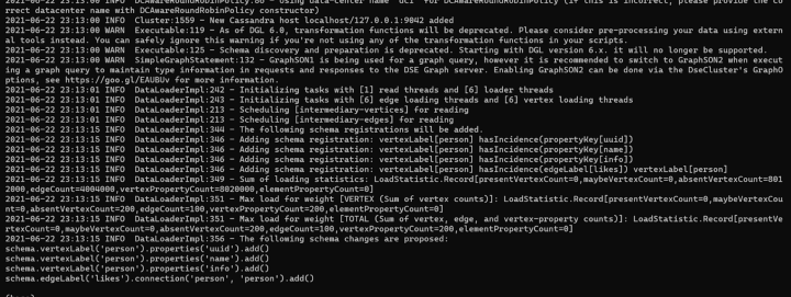
For each of our trials, we will create four supernodes, each with 1 million edges. DSE GraphLoader gives the following output:

The output shows 4,000,000 edges, which confirms that we ingested the correct amount of edges.
Step 3: Confirm Edge Count in Gremlin
We can take the ID of one of our supernodes to test whether there are indeed 1 million incident edges for this supernode:

Looking good so far!
Step 4: Confirm Wide-partitions in Cassandra
Next, let’s check to make sure we really do have a wide partition as expected. Note that we will want to make sure we flush to disk using nodetool flush to ensure that everything is in sstables so that our tablestats will give us numbers that reflect all of our records. Then we can use tablestats to get partition sizes.
Vertices table (Table: person_p) partitions should not be large – each uuid is its own partition key, so those vertices should each basically have their own partition:
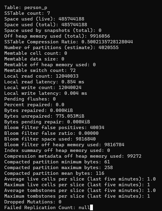
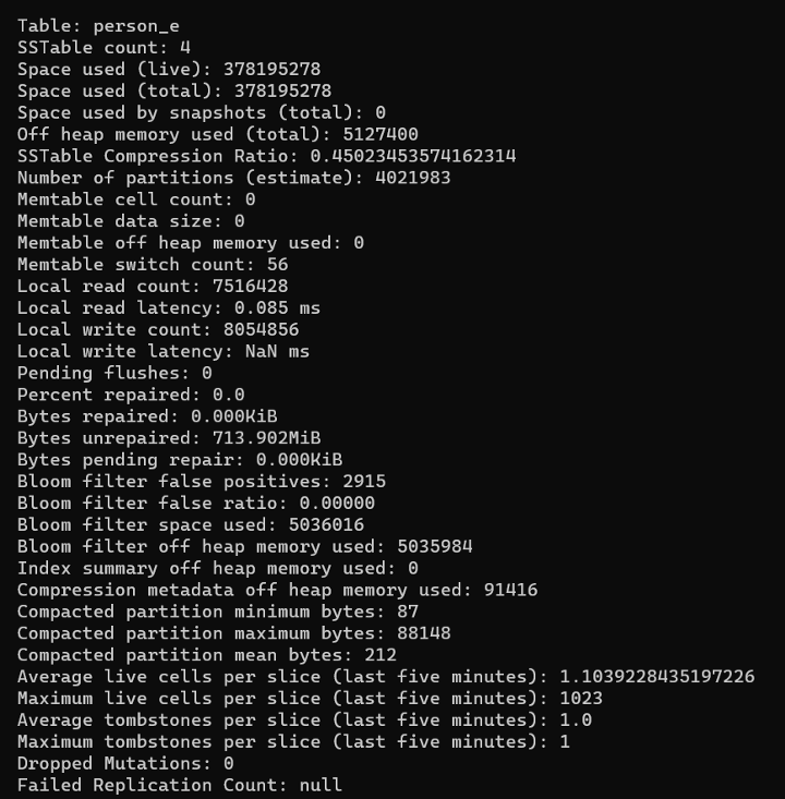
The edges table (person_e) however should have large partitions, since each supernode should have all 1 million edges grouped together with it:
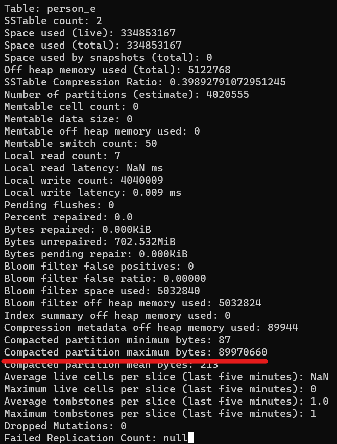
As you can see, the output reads “Compacted partition maximum bytes” of 89,970,660 and “Space used (total)” of 334,853,167. This matches our expectations: 80+ MB/partition and four times that for total disk space used since we created four supernodes.
Step 5: Verify shape of graph in DSE Studio
Before moving on to our next trial run where we try out intermediary vertices, it’s worth taking a moment to visualize our graph in DSE Studio. DSE Studio only shows 1000 elements at a time, so we shouldn’t rely on this too heavily for our experiment, but still, it can at least help us get a mental image of what’s going on here. Note also that some of the Gremlin traversals shown below are not written for performance but rather just to make sure it displays correctly in DSE Studio.
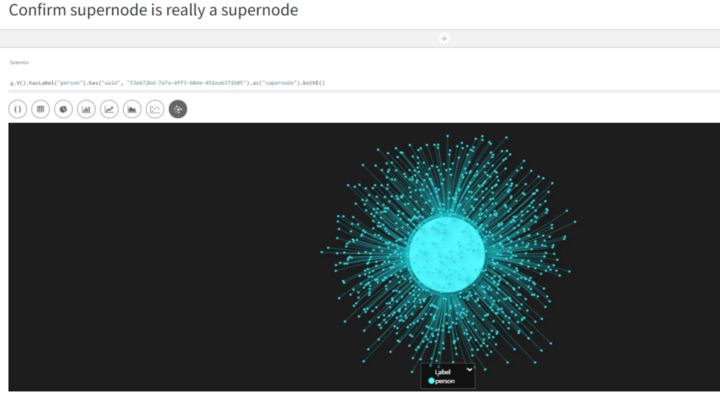
Visualize a supernode
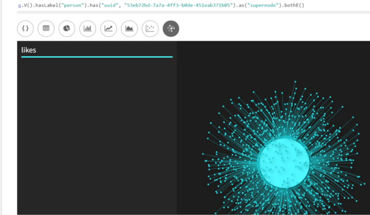
Going out from one of our supernodes, we can see how there is one central node (the big one) to which all other nodes are connected.
g.V().hasLabel("person").has("uuid", "53eb72bd-7a7a-4ff3-b0de-451eab371b05").as("supernode").bothE()
Trial #2: Try to Break Apart Supernodes Using Intermediate Vertices
Next, we will try out intermediate vertices, the solution mentioned in our previous post. The idea is that by introducing a vertex in between our supernode and its adjacent vertices, we can keep partition sizes manageable, as suggested by a DSE Graph team member here in this StackOverflow post.
Step 1: Create schema
Our schema for this will be the same as in the first trial: a simple vertex person with an edge called likes.
Step 2: Send CSV data using DSE GraphLoader
As in the previous step, we ingest the CSV data, but this time the data has a different shape. Each supernode still has 1 million other persons who “like” them as before, but for each supernode, we introduce 1000 intermediary vertices, each of which has 1000 terminal vertices.
Looking at our CSV with the edges that we will use for ingestion, there are indeed 4,004,000 edges: 4,000,000 from the intermediary vertices to the end vertices, and then 4000 from the supernodes to the intermediary vertices.
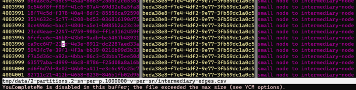
Load intermediary vertices into DB using DSE GraphLoader
Step 3: Confirm Edge Count in Gremlin
If our test worked, the “supernodes” should no longer have wide partitions. Incident edges should be down to 1000 per supernode, whereas before it was 1,000,000.
When we can use the same Gremlin traversal that we did in Trial #1. In trial #1, this traversal returned 1 million incident edges for this supernode. Now it should only return the intermediary vertices, so as expected there are only 1000:

Make sure this is true for all supernodes
By assigning the supernode uuids to a variable sn_uuids, we can confirm that all supernodes are the same. As expected, there are four supernodes, each with 1000 (= 4000 edges).

Go out two hops and make sure we’re getting some people
Our previous traveral confirmed that each supernode has 1000 intermediary vertices. Let’s go out from one of these intermediary vertices, and make sure there are 1000 terminal vertices on the other side.

Step 4: Confirm Smaller Partition Size in Cassandra
Finally, the moment of truth. We again flushed to disk and then used tablestats to check partition size. As we were hoping for,, the edges table (person_e) no longer has large partitions.
“Compacted partition maximum bytes” comes out to 88148, which is roughly 89 KB. This is roughly 1000x smaller than the result from the first trial (roughly 89 MB).
And just for a sanity check, we also see that total disk space is roughly the same, though slightly higher (since we introduced 1000 new vertices and their edges). Now, “Space used (total)” comes out to around 370 MB, whereas before it was around 330 MB.
Step 5: Verify shape of in DSE Studio
As noted before, we have to be careful here, since DSE Studio shows a maximum of 1000 vertices anyways. This means that the original supernode will look more or less the same since it still has 1000 incoming edges:
As expected, still has a lot of connections. Even still, the visualization can help us see what’s going on here a little bit.
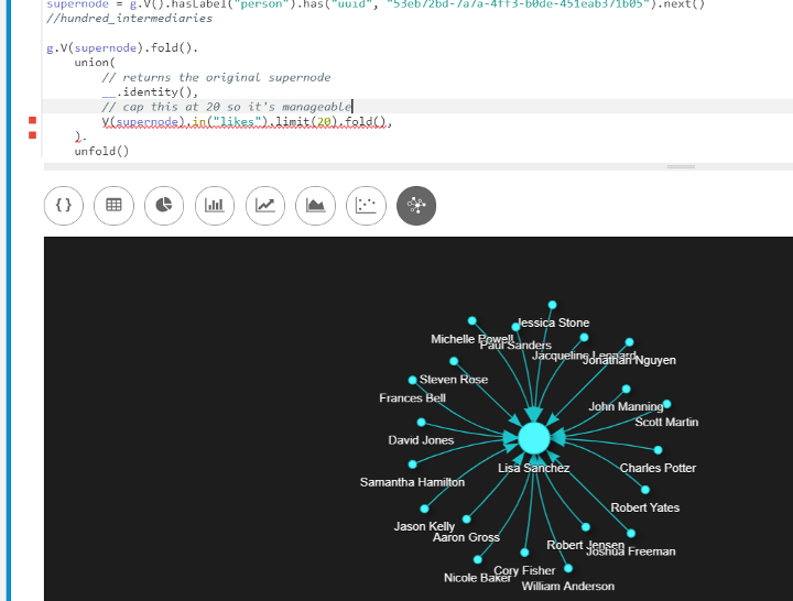
What we can do is look at only the supernode with 20 of its intermediary vertices, so that we can visualize how this thing looks without hitting the 1000-element maximum. (We are using fold and union steps as well here in order to make sure it looks nice in DSE Studio). Before expanding, it looks like this:
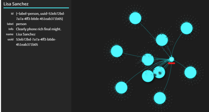
Using “Expand neighborhood” feature, we can get a better idea of how this graph looks
The “Expand neighborhood” feature makes it easy to go out from nodes found in a traversal within DSE Studio. Using this feature, we go out another hop and see how the supernode (underlined in red below) is connected to intermediary vertices (due to the 1000 element limit, only 10 are shown now), which in turn are connected to several others.
Conclusion
Overall, our experiment was successful. We showed how supernodes create wide partitions in DSE Graph, and how to break those wide partitions up using intermediary vertices. While this means we use a little higher total disk space, the partition size can become much more manageable.
It bears repeating though that this solution is less than ideal for several reasons. As mentioned in the previous post, not only is there an “edge cut” (i.e., traversals from one vertex to its adjacent vertex require crossing partitions, adding network latency, etc), but there is also an extra hop involved in order to get from your source note to your destination node, since now there is this “intermediate vertex” in between. This also adds greater complexity to your applications’ business logic if they ever do run these traversals.
This brings us to our alternative solution for breaking up supernodes in DSE 6.7: you guessed it, upgrading to DSE 6.8. This will be the focus of the final post of this series.
Series
- Partitioning in DSE Graph
- Solving Wide Partitions caused by Supernodes in DSE 6.7
- Solving Wide Partitions caused by Supernodes in DSE 6.8
Cassandra.Link
Cassandra.Link is a knowledge base that we created for all things Apache Cassandra. Our goal with Cassandra.Link was to not only fill the gap of Planet Cassandra but to bring the Cassandra community together. Feel free to reach out if you wish to collaborate with us on this project in any capacity.
We are a technology company that specializes in building business platforms. If you have any questions about the tools discussed in this post or about any of our services, feel free to send us an email!