Introduction
In the first part of this blog series, we looked at the underlying issue that supernodes cause in DSE Graph due to how partitioning in Cassandra works and solutions that have been put forward for DSE Graph 5.x and 6.0-6.7. In the second part, we took a look at what this actually looks like within DSE 6.7 via some hands-on experimentation with intermediary vertices. We saw that although intermediary vertices successfully break apart the wide partitions, there are some problems inherent in introducing an extra hop like that.
In this third and final part of the series, we will look at how we can take advantage of the changes made in DSE 6.8 in order to implement a better solution than what was possible in DSE 6.7.
What changed in DSE Graph 6.8
I will leave it to you to read the release notes for DSE 6.8 yourself, but this quote from the Datastax blog gives a good overview to get us started:
With DSE 6.8, DataStax is taking the next step in the evolution of distributed graphs by moving the graph storage engine deeper into Cassandra.
Now in DSE 6.8, the Tinkerpop graph vertices and edges can be read or written from either Gremlin or CQLSH. You can even take an existing Cassandra keyspace and turn it into a graph by running some alter statements. All of this is on top of a reported 10 times faster performance boost. (Of course, saying “10x faster!” is kind of vague and I can’t tell you precisely what it means, but you know it has to be good!)
There are many interesting implications of the changes that they made here, but for our particular use case, we see that DSE 6.8 allows us to solve wide-partition issues caused by supernodes in a much more elegant way than intermediate vertices. In DSE 6.7 we could control the partitioning of vertices by way of custom vertex ids, but we had no way to partition the edges directly. Now in DSE 6.8 however, since we can specify the edges’ the primary key as they are actually stored in Cassandra, we are able to partition the edges as needed.
When creating the schema using Gremlin, this is accomplished by using .partitionBy() and .clusterBy(). If you don’t use these steps, the default behavior is that the Cassandra table for these edges will have a primary key based on the origin (aka outgoing) side of the edge. In other words, if son isChildOf father, then by default, the isChildOf edge would have a partition key that is based on the son vertex. If you use .partitionBy however then you can choose a different property instead.
As an aside: It is worth noting that regardless, you will need to include the columns of the primary key of both the origin and destination vertex within the primary key of the edge, however. When you think about how edges work in Tinkerpop and how primary keys work in Cassandra, this makes sense. In Tinkerpop, an edge needs to be associated with a particular origin vertex and destination vertex and these cannot be changed (to “change” which vertex an edge is associated with, you just have to drop it and make a new one). Accordingly, using the primary keys in Cassandra (which are themselves immutable) to associate the edge with particular vertices is quite logical. All that to say: be careful of this when thinking about picking your primary keys for these vertices and edges. As always, picking the right primary key is crucial for your data model in Cassandra.
Anyways, for our use case, the important thing is that now we can divide up our edges for our supernode into different partitions without intermediate vertices: all we have to do is add some other property to our edge’s partition key.
Our approach
Our general process will be the same as what we did in part two. We will be using code from the same repo as before for setting up our experiment: https://github.com/Anant/dse-graph-supernode-generator. We will also likewise start with a control by creating the supernode using default partitioning behavior, and then we will show how to solve the wide-partition issue with our proposed solution.
Trial #1: Control
For our control, we will set up a graph similar to before, but due to default behavior in DSE 6.8, the direction of the edges needs to be in reverse order for our experiment to work correctly. By default edge partitions are based on the partition key of the origin vertex, rather than duplicated and stored with both vertices like before. Unfortunately, I learned about this behavior the hard way. I haven’t found official documentation that discusses this point, but it was confirmed in the comments of this Datastax Community answer.
This won’t make a major difference for us, but just note that our supernode will not be “liked” by 1 million people, rather they will “like” 1 million other people instead.
Step 1: Create schema
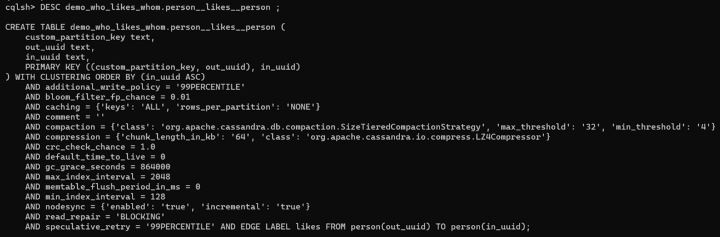
Even though we create the same vertices and edges schema as we did for DSE 6.7, the outcome in CQLSH is pretty different, and for the better.
Notice that there are no extra fields beside the primary key in the properties that we specified. Again, this was done intentionally by the developers of DSE 6.8 in order to make it possible to query your entities using CQL or Gremlin interchangeably.
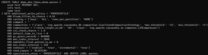
person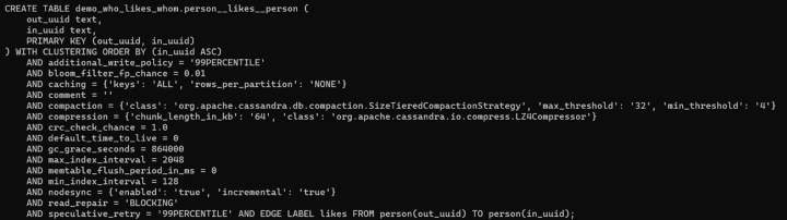
person__likes__person Also, note that while the primary key of the edge refers to the primary keys for both the origin vertex (out_uuid) and the destination vertex (in_uuid), the partition key of the edge is out_uuid, not in_uuid. This aligns with what we mentioned above, that the default behavior for edges is that they are stored in with the origin vertex.
Step 2: Send CSV data using DSE Bulk Loader
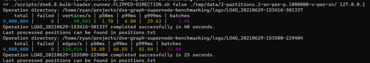
Now that we are using DSE 6.8, we will also use DSE Bulk Loader instead of DSE GraphLoader. There are various advantages to this, but for our case, the result is the same: we load in our data and we are left with some brand new supernodes.
Here is the output when loaded in the sample data from the generated CSV:
Step 3: Confirm Edge Count in Gremlin
Using a Gremlin traversal, we can confirm that our supernode “likes” 1 million other people:

So far so good!
Step 4: Confirm Wide-partitions in Cassandra
Let’s also just quickly confirm that we really did make some wide partitions here. Just like we did for DSE 6.7, we again flushed to disk and then used tablestats to check partition size.
The vertex table (person) is more or less what we expected, with many small partitions for the vertices: 4,014,418 estimated partitions, with “Compacted partition maximum bytes” of 179 bytes.
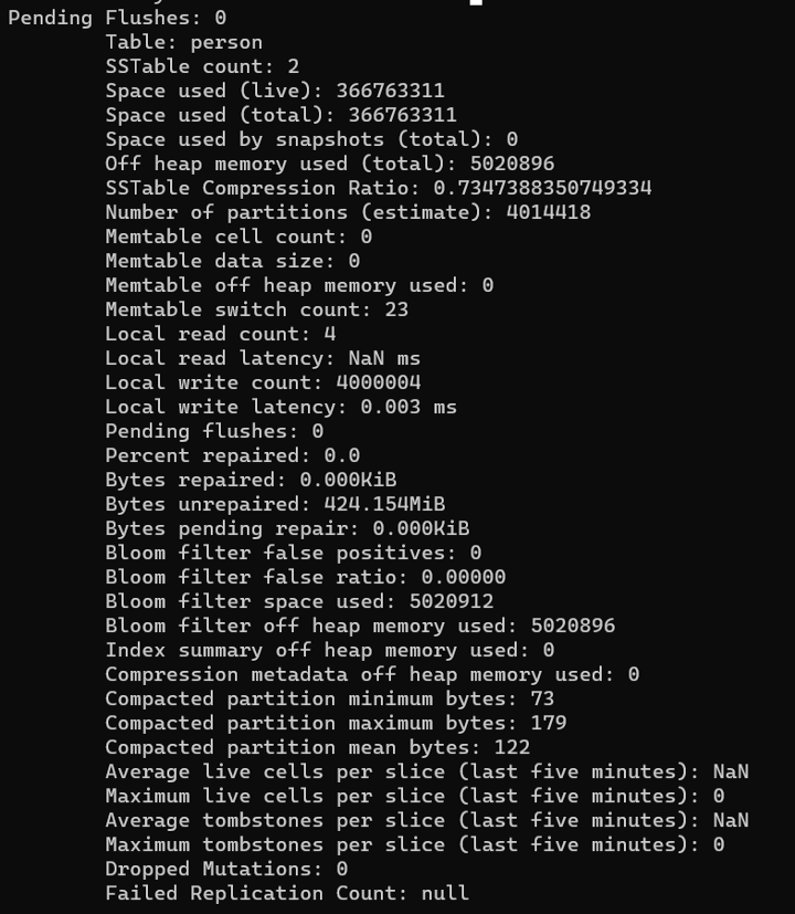
One unexpected result though was that the “Space used (total)” came out to around 366 MB instead of the 485 MB that we saw in our DSE 6.7 control trial.
Turning then to the edge table (persion__likes__person), we can see some other interesting results:
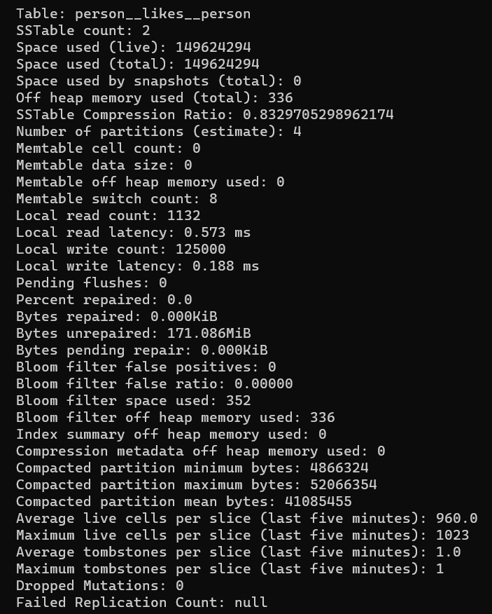
As was the case for vertices, the total space used (149,624,294 bytes, around 149 MB) is less than what we saw in DSE 6.7 – around 334 MB, almost twice as much. In other words, the data stored in DSE 6.8 appears to be half as much, at least for this sample. This was unexpected, but a possible explanation for why is that there are some extra fields that get added to the partition key automatically in 6.7. Perhaps this is part of how DSE 6.8 delivers that advertised “10x performance” boost.
In regard to partitions, here we see there are four partitions (one per supernode), and a “compacted partition maximum bytes” of 52,066,354 bytes (roughly 52 MB). This is smaller than the size of partitions we had for test control for 6.7 (around 90 MB), but this makes sense as well given that it seems like the edge records are taking half the size. Of course, these are not really very wide as far as partitions go, but at least we have a number that we can refer to for the sake of testing.
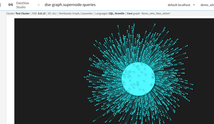
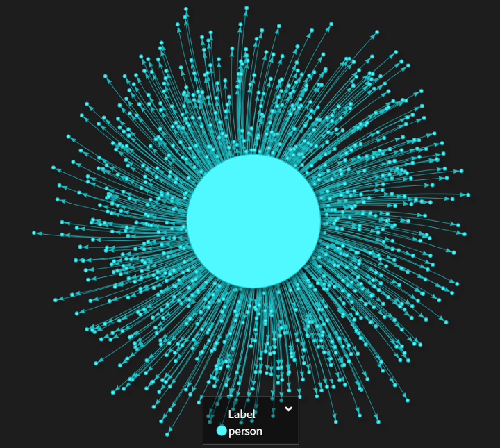
Step 5: Verify shape of graph in DSE Studio
When we visualize the shape of the graph in DSE Studio, we see a similar shape to what we saw for our experiments regarding DSE 6.7, though now our arrows are going in a different direction since our edges are going out from the supernode instead of in.
Now that we have confirmed that we have some supernodes and wide partitions (or at least, wide enough for testing against), we can move on to our final trial, where we will attempt to break apart the wide partitions using the
Trial #2: Try to Break Apart Supernodes Using Partition Keys
Step 1: Create schema
We can keep the same schema for vertices, but we will add another column to our edge table’s partition key:
Now our primary key looks like this:
PRIMARY KEY ((custom_partition_key, out_uuid), in_uuid)
The out_uuid field is still part of the partition key, but now it is part of a composite partition key along with another field, custom_partition_key.
Step 2: Send CSV data using DSE Bulk Loader
Now that we have a schema, we are ready to load our data using DSE Bulk Loader.
Here is the output for loading our 4 supernodes with 1 million edges each:

Step 3: Confirm Edge Count in Gremlin
I started to get a little more creative with my Gremlin traversals here, but the result is still the same: 1 million edges per supernode.
supernodes = g.with('allow-filtering').V().hasLabel("person").has('uuid', within(sn_uuids)).project('supernode_id', 'people-whom-they-like').by(id).by(outE("likes").count())

Step 4: Confirm Smaller Partition Size in Cassandra
And finally, the moment of truth: tablestats for edge table (person__likes_person)
Here we see that the estimated number of partitions comes out to 4000. This makes sense, since we have four supernodes, each with 1,000,000 adjacent vertices, and they were divided into partitions with 1000 edges max per partition.
The compacted partition maximum bytes comes out to 51,012 (around 50 KB). Success! This is roughly 1000x less than what we saw for our test control, which had partitions of roughly 52 MB, matching our expectations, since we divided up edges so that there were 1000 edges per partition.
If we visualize in DSE Studio, we see that the shape of the graph is unchanged.
Conclusion
My hope is that by running through this exercise, it helps to clarify the differences between DSE Graph 6.7 and 6.8, and how you would go about splitting apart wide partitions caused by supernodes in both versions. The solution that we see here for DSE 6.8 has several advantages over introducing intermediary vertices like we had to do for DSE 6.7, but perhaps what is most appealing is its simplicity. There would be no extra hop when traversing from the supernode, and therefore there would not be any code changes required either.
However, it is worth noting that this does not solve everything. In particular, this solution still introduces “edge cut” since the edges are no longer co-located with the vertex. This is a trade-off that you will have to weigh out depending on your traversal patterns and how wide your partitions are. Thank you for following along with the Wide partitions and supernodes in DSE Series. If you missed parts 1 and 2, they are linked below.
Wide partitions and Supernodes in DSE Series
- Partitioning in DSE Graph
- Solving Wide Partitions caused by Supernodes in DSE 6.7
- Solving Wide Partitions caused by Supernodes in DSE 6.8
Cassandra.Link
Cassandra.Link is a knowledge base that we created for all things Apache Cassandra. Our goal with Cassandra.Link was to not only fill the gap of Planet Cassandra but to bring the Cassandra community together. Feel free to reach out if you wish to collaborate with us on this project in any capacity.
We are a technology company that specializes in building business platforms. If you have any questions about the tools discussed in this post or about any of our services, feel free to send us an email!